

Introduction
In Part 3 – Teaching the machine, I described two important approaches used in the training of artificial neural networks. Both of these approaches involved a certain amount of intervention to point the network towards the required solution. The first, back-propagation was mathematically robust but limited in scope. The second, Hebbian learning, was more aligned to what happens in biological brains, but harder to direct towards a tightly specified outcome.
As an analogy, you can steer your car to exactly where you want it, or you can design it to steer itself and ride along as a nervous passenger. Either can get you to where you want, but not necessarily by the route you choose.
However, there is a third way, and something that plays an important part in the learning process in you and me. It’s called competitive learning, and it’s how we learn to group similar things into categories. You could also call it stereotyping. It’s important, because without these groupings, animals would have to deal with every encounter as if it were the first time. Previous experience would mean very little, and we’d struggle to survive.
Survival of the fittest
So, what is competitive learning, and what does it do for us? Despite its name, it hasn’t got anything to do with competing with other neural networks. It’s all about the brain competing with itself. One of the biggest differences with this approach is that it can happen without any outside intervention. No desired output is needed and no reward is required. The network just gets on with the process of putting things in boxes.
To perform this magic, we need to build a new type of neural network, known as an auto-associative memory. If you’ve ever heard of a Hopfield Network, then you’ve heard of at least one type of these specialised machines. Brains are very efficient at using just enough neurons to achieve an outcome, leaving the rest free for further experiences. Auto-associative networks are an attempt to duplicate this.
This is where competitive learning comes in. In this type of learning, we don’t care which neurons fire. We just want to make sure only a few fire for each situation, and different ones fire when the situation changes.
The winner takes it all
The way this is achieved is through a winner-takes-all approach. Neurons are connected in such a way that the strongest firing neuron provides positive feedback to its nearest neighbouring neurons and negative feedback to those neurons that are further away. Each input is then connected to all of these neurons, so each one gets a chance to respond to the input pattern based on its initial weights.
The following diagram shows a simplified representation of such a network. Connectivity from all inputs to all neurons, and connectivity from one neuron to all other neurons is shown. Close neighbours are connected with a positive weight and distant neighbours with a negative weight. The graph below shows how connection weight varies with distance for a larger network. Because of the shape of this graph, it is often referred to as a “Mexican hat” weight distribution.

When patterns of inputs are first presented to a network like this, each neuron fires at a different level depending on how closely its weights match the inputs. The neuron that best matches the pattern then “recruits” its nearest neighbours via positive feedback and they start to fire more strongly as well. Meanwhile, neurons further away are forced to fire less strongly due to the negative feedback that they receive from the original neuron and its new recruits.
As a result, the neurons compete with each other. The strongest groups get even stronger and the weaker groups fade away. Hebbian learning is then used to adjust the weights of the neurons based on their inputs and firing rates. (I discussed Hebbian learning in Part 3 – Teaching the machine). This learning approach strengthens the weights that match the input pattern for the neurons that fire the most. Inputs that don’t match the pattern are weakened as a result of the decay factor built into Hebbian learning.
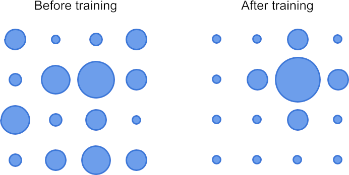
The diagram above shows an example of this in a simple, 16 neuron auto-associative memory. Each circle represents a neuron and the sizes of the circles represent their relative firing rates. Before training, when a pattern is presented, firing rates are varied, and a clear winner is not necessarily obvious (left hand side of diagram). Over time, one winning group emerges and a single neuron dominates (right hand side of diagram).
In the future presentations of this pattern, only this neuron and its immediate neighbours will respond to this particular pattern. When a new pattern is presented that is different to the first, the winning neurons from the first round fire weakly because they have become specialised to one pattern. The rest of the neurons fire at varying levels, and take part in the competition to claim this new pattern.
A place for everything
As more patterns are presented to the network, more of these small neuron groups are created and eventually you have a network that can respond to each pattern by firing only a very small number of neurons. This is known in AI as sparse encoding, and it’s one of the things that makes the biological brain so energy efficient.
An added advantage of this approach is that similar patterns end up getting represented by neuron groups that are close to each other, and different patterns are separated from one another. The network is even capable of classifying things it has never seen before, simply because they are most like something it has seen. The network has become a classifying machine based solely on the inputs. We, its creators, have not needed to intervene in the process.
In biological brains you can observe this happening. Present a patient with the sound of a barking dog, and a scan will show specific neurons firing. Present the same patient with a piece of orchestral music and very different sets of neurons will fire. It is not unreasonable to suggest that these groups represent your memories.
A side effect of this process is stereotyping. The brain is inherently biased by design, especially with respect to groups it has limited exposure to. I touched on this in a previous blog post, AI washing and the prejudiced machine.
A bit of a brain
So, that’s auto-associative memory. It allows networks to learn even when there’s no desired output or action, it helps brains to be highly energy efficient, and it could well be how experiences are remembered. No mean feat for such a simple concept.
However, it has a limitation. This type of network can’t be used to create a problem solving artificial brain on its own, any more than an engine will get you to work. It’s just a specialised component, but it is a rather important one.
It’s also possible that this autoassociative behaviour isn’t just taking place in one part of a biological brain. Experimental observations suggest that this type of competitive learning is happening throughout the brain.
Onwards, fellow Frankensteins!
So far, I’ve covered artificial neurons, two types of neural network, and a process for classifying and remembering experience. In the next part, things are going to get biological. It’s time to revisit that simple artificial neuron and make it more sophisticated.
I’ll talk a about something known as “biological plausibility”, delve a bit deeper into how a real neurons behaves, and explain a model I’ve developed that’s a bit more brain-like.
Why? Because the more like a real neuron we can make it, the more chance we have of adding the intelligence to the artificial.